The Perceptron: AI’s First Step

About the Perceptron

The Perceptron represents the very first chapter in the history of artificial intelligence. Its development was sparked by a simple but profound line of questioning:

1. “How does the human brain learn?”
2. “It seems to be composed of units called neurons.”
3. “Therefore, to create an ‘Artificial Intelligence,’ we should try to build an artificial neuron.”

This idea, to model the biological processes of the brain, was the seed from which the field of machine learning grew.

---

Early Models of Artificial Neurons

In the beginning, AI research was heavily focused on mathematically modeling the human brain to create this “artificial neuron.” This led to several key conceptual milestones.

1. McCulloch & Pitts Neuron (1943)

A LOGICAL CALCULUS OF THE IDEAS IMMANENT IN NERVOUS ACTIVITY , McCulloh and Pitts

This was a highly simplified, foundational model.

• It received binary inputs (0 or 1).
• It computed a weighted sum of these inputs.
• It would “fire” (output 1) if this sum exceeded a certain threshold, and output 0 otherwise.
• Crucially, McCulloch and Pitts demonstrated that by combining these simple units, one could create any Boolean logic gate (like AND, OR, NOT).

2. Hebb’s Learning Rule (1949)

The Organization of behavior a neuropsychological theory

Donald Hebb introduced a concept that became a cornerstone of learning:

“Neurons that fire together, wire together.”

Inspired by how synapses in the brain strengthen with repeated use, Hebb proposed a learning rule where the weight (the connection strength) between neurons is not fixed but changes over time. If two neurons are frequently active at the same time, the connection between them strengthens.

3. Rosenblatt’s Perceptron (1957)

The Perceptron

Building on these ideas, Frank Rosenblatt introduced the Perceptron. This was not just a static model but a learning algorithm. It introduced an automated way for the model to learn the optimal weights from data, which is widely considered the beginning of machine learning as we know it.

---

What is a Perceptron? A Linear Classifier

The Perceptron is, fundamentally, a linear classifier for binary classification.

This means it learns to separate data into two distinct classes by finding a linear boundary.

• In a 2D space, this boundary is a line.
• In a 3D space, it’s a plane.
• In higher-dimensional spaces, it’s called a hyperplane.

The Perceptron’s job is to learn the “best” line (or hyperplane) to separate the two groups of data points.

---

Structure of a Perceptron

A Perceptron has several key components that mimic its biological inspiration.

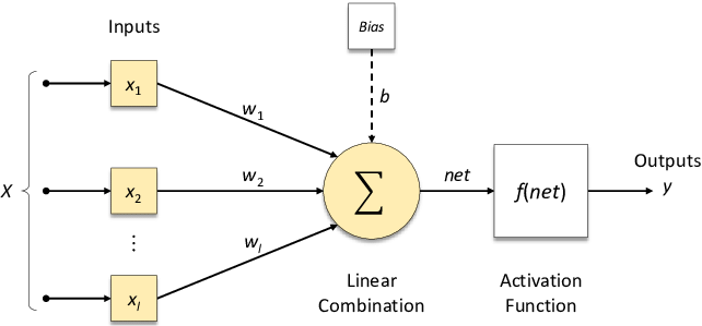
(img from researchgate)

• Inputs ($x_1, x_2, \dots, x_n$): The features of a single data point.
• Weights ($w_1, w_2, \dots, w_n$): Adjustable parameters that represent the importance or strength of each input.
• Summation ($\Sigma$): A weighted sum of the inputs, plus a bias term.
• Activation Function (Step Function): A function that processes the sum and produces the final output.
• Output ($y$): The final prediction (e.g., -1 or 1, or 0 or 1).

---

Biological Analogy:

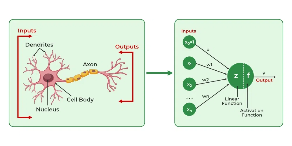
(img from GeeksforGeeks)

• Inputs / Weights are like Dendrites (which receive signals of varying strengths).
• Summation / Activation is like the Nucleus/Soma (which processes the signals).
• Output is like the Axon (which transmits the final signal).

The model we’ve just described, with one set of inputs and one output, is a Single-Layer Perceptron (SLP). When we stack these perceptrons into multiple layers (with hidden layers between the input and output), it becomes a Multi-Layer Perceptron (MLP).

The Mathematical Model

The Perceptron computes a weighted sum $z$ of its inputs.

\[ z = w_1x_1 + w_2x_2 + \dots + w_nx_n + b \]

Where $b$ is the bias term. The bias shifts the decision boundary off the origin. We can simplify this by including the bias as a weight $w_0$ whose corresponding input $x_0$ is always 1.

\[ z = \sum_{i=0}^{n} w_i x_i = \mathbf{w}^T \mathbf{x} \]

This sum $z$ is then passed through an activation function, which in the classic Perceptron is a step function (or sign function). This function determines the final output.

\[h_{\mathbf{w}}(\mathbf{x}) = \text{sign}(\mathbf{w}^T \mathbf{x}) = \begin{cases} 1 & \text{if } \mathbf{w}^T \mathbf{x} \ge 0 \\ -1 & \text{if } \mathbf{w}^T \mathbf{x} < 0 \end{cases}\]

If the weighted sum is positive or zero, the neuron “fires” and outputs 1. If it’s negative, it outputs -1.

---

Perceptrons as Logic Gates

A Single-Layer Perceptron can represent several basic boolean logic gates. Let’s assume inputs $x_1, x_2 \in {0, 1}$ and an activation function that outputs 1 if $z \ge 0$ and 0 otherwise.

AND Gate

Outputs 1 only if $x_1 = 1$ AND $x_2 = 1$.

• Weights & Bias: $w_1 = 1$, $w_2 = 1$, $b = -2$
• Logic:
  • $x_1=0, x_2=0 \to (1 \times 0) + (1 \times 0) - 2 = -2 \to 0$
  • $x_1=1, x_2=0 \to (1 \times 1) + (1 \times 0) - 2 = -1 \to 0$
  • $x_1=0, x_2=1 \to (1 \times 0) + (1 \times 1) - 2 = -1 \to 0$
  • $x_1=1, x_2=1 \to (1 \times 1) + (1 \times 1) - 2 = 0 \to 1$

OR Gate

Outputs 1 if $x_1 = 1$ OR $x_2 = 1$.

• Weights & Bias: $w_1 = 1$, $w_2 = 1$, $b = -1$
• Logic:
  • $x_1=0, x_2=0 \to (1 \times 0) + (1 \times 0) - 1 = -1 \to 0$
  • $x_1=1, x_2=0 \to (1 \times 1) + (1 \times 0) - 1 = 0 \to 1$
  • $x_1=0, x_2=1 \to (1 \times 0) + (1 \times 1) - 1 = 0 \to 1$
  • $x_1=1, x_2=1 \to (1 \times 1) + (1 \times 1) - 1 = 1 \to 1$

NOT Gate

Outputs the opposite of the single input $x_1$.

• Weight & Bias: $w_1 = -1$, $b = 0$
• Logic:
  • $x_1=0 \to (-1 \times 0) + 0 = 0 \to 1$ (Outputs 1 for $z \ge 0$)
  • $x_1=1 \to (-1 \times 1) + 0 = -1 \to 0$

---

Training a Perceptron

How does the Perceptron learn the right weights ($\mathbf{w}$)? It uses a simple iterative algorithm.

The Perceptron Learning Algorithm

1. Initialize: Start with weights $\mathbf{w}$ (e.g., all zeros or small random values).
2. Iterate: For each training example $(\mathbf{x}_n, y_n)$ from the training set:
   • a. Predict: Calculate the output $\hat{y} = \text{sign}(\mathbf{w}^T \mathbf{x}_n)$.
   • b. Check for Mistake: If the prediction is wrong ($\hat{y} \ne y_n$), update the weights.
3. Repeat: Loop through the dataset multiple times until no more mistakes are made (the model has converged).

The Update Rule

The core of the learning is the update rule, which is applied only when a mistake is made:

\[ \mathbf{w} := \mathbf{w} + y_n \mathbf{x}_n \]

Let’s analyze this (assuming true labels $y_n$ are ${-1, 1}$):

• Case 1: False Negative.
  • The true label is $y_n = 1$.
  • We predicted $\hat{y} = -1$ (because $\mathbf{w}^T \mathbf{x}_n < 0$).
  • The update is: $\mathbf{w} := \mathbf{w} + (1)\mathbf{x}_n = \mathbf{w} + \mathbf{x}_n$.
  • This adds the input vector $\mathbf{x}_n$ to the weights. This pushes $\mathbf{w}$ to be more similar to $\mathbf{x}_n$, making the dot product $\mathbf{w}^T \mathbf{x}_n$ larger (more positive) and more likely to be correct next time.
• Case 2: False Positive.
  • The true label is $y_n = -1$.
  • We predicted $\hat{y} = 1$ (because $\mathbf{w}^T \mathbf{x}_n \ge 0$).
  • The update is: $\mathbf{w} := \mathbf{w} + (-1)\mathbf{x}_n = \mathbf{w} - \mathbf{x}_n$.
  • This subtracts the input vector $\mathbf{x}_n$ from the weights. This pushes $\mathbf{w}$ to be less similar to $\mathbf{x}_n$, making the dot product $\mathbf{w}^T \mathbf{x}_n$ smaller (more negative) and more likely to be correct next time.

This algorithm is guaranteed to find a solution (a separating hyperplane) if the data is linearly separable.

Loss Function (Perceptron Criterion)

This update rule is effectively performing Stochastic Gradient Descent (SGD) on the Perceptron loss function. This loss is zero for correctly classified points and positive for misclassified ones.

\[ L(\mathbf{w}, \mathbf{x}_n, y_n) = \max(0, -y_n (\mathbf{w}^T \mathbf{x}_n)) \]

For a misclassified point, $y_n$ and $\mathbf{w}^T \mathbf{x}_n$ have opposite signs, so their product is negative. The loss is then $-y_n (\mathbf{w}^T \mathbf{x}_n)$, which is a positive value.

For a correct point, the product is positive, so the loss is $\max(0, \text{negative value}) = 0$.

---

Limitations of the Perceptron

The Perceptron’s simplicity is also its greatest weakness.

A Single-Layer Perceptron can only solve problems that are linearly separable.

This means it fails spectacularly if the data classes cannot be separated by a single straight line.

The XOR Problem

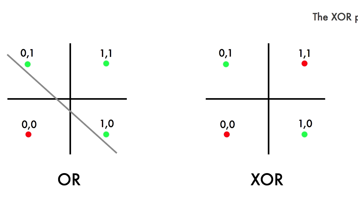(img from DEVcommunity)

The most famous example of this limitation is the XOR (Exclusive OR) problem.

The XOR gate outputs 1 if the two inputs are different, and 0 if they are the same.

$x_1$	$x_2$	Output
0	0	0
0	1	1
1	0	1
1	1	0

If you plot these four points on a 2D graph (with (0,0) and (1,1) as one class, and (0,1) and (1,0) as the other), you will find it impossible to draw a single straight line to separate the ‘0’s from the ‘1’s.

This limitation, famously highlighted by Minsky and Papert in 1969, led to a significant decline in AI research, an era known as the first “AI winter.”

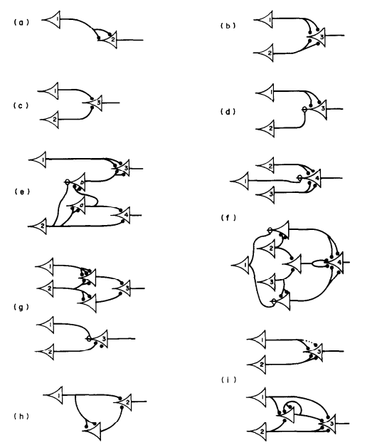
The Solution: Depth

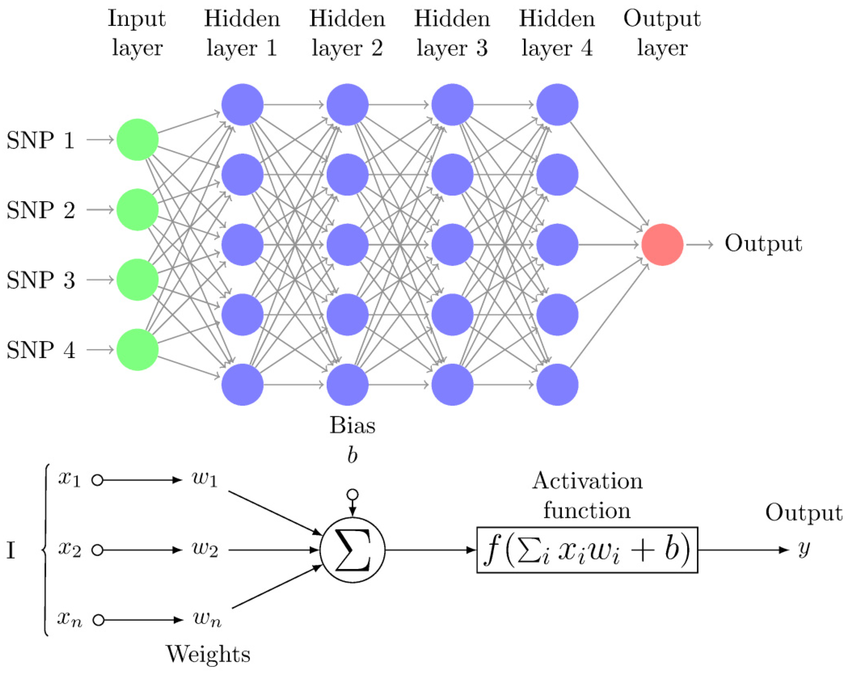(img from ResearchGate)

The solution to the XOR problem, and the key to unlocking the power of neural networks, is the Multi-Layer Perceptron (MLP). The figure above shows an MLP with four hidden layers.

By stacking layers of perceptrons and introducing non-linear activation functions (like Sigmoid or ReLU), an MLP can learn complex, non-linear decision boundaries. An MLP can easily solve the XOR problem, and this architecture forms the foundation of modern deep learning.